
How to Swap Solver Types
From Version 2.14 onwards, our new V3 Optimizer is the default option assigned to newly created projects. This solver is in general substantially faster and more transparent than the previously available Full Optimization methods. Pre-existing projects may also have this solver assigned to it (or its Equal Well Const By Pad twin), whereby pending the particular pipeline configuration, some adjustments may be required in order to facilitate getting the same answer.
This topic outlines the recommended testing and review process to assist in converting from your currently selected solver to our new and improved version. As a part of this process you may need to adjust inputs to retain the currently achieved results.
Is this a Candidate Model?
The first check before proceeding on an adjustment of the solver option is to verify if you are sufficiently happy with the results of the model within 2.14 using the currently selected solver option (note that within this update there are some expected regressions from previous results). Note that general guidance on comparing models is specified below.
The second check is whether the model complies with a couple of the limitations of the new option, specifically confirming that neither of the two items below exists:
- Extraction rates are above 100%. This may be easily checked by selecting Byproducts All or Extraction All then reviewing what the facility extractions are, noting that H2S, CO2, Inert and Water are always extracted regardless of the extraction/yield checkbox
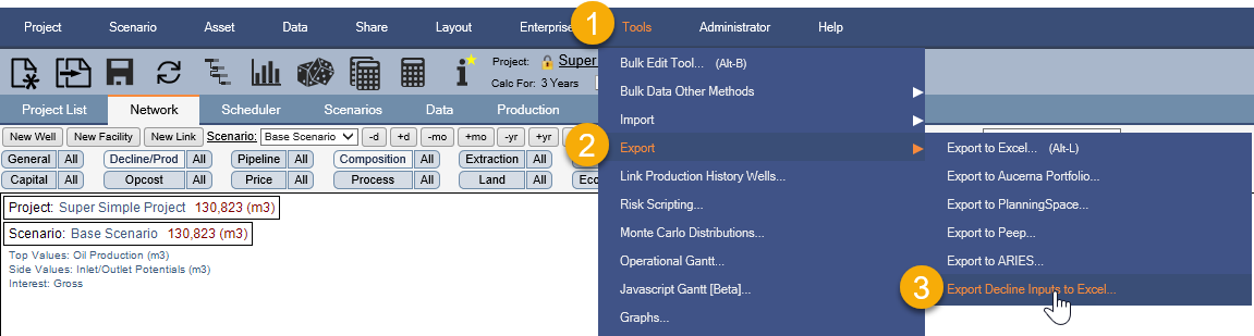
- Negative production exists. This may be checked via exporting the Decline inputs to Excel for each scenario then reviewing the resultant excel file for any negative inputs.
- Energy Constraints with WI only pipelines and Heating Value Overrides. This may be checked by selecting Constraints All and seeing if any Energy constraints (HeatingValue or HeatingValuePerVolume) have been specified in addition to also checking Pipeline All to see if any connections have ‘WI Flow’ checked then finally checking Composition All to see if the heating value has ‘override’ specified for any wells.

Click image to expand or minimize.
Click image to expand or minimize.
The third check only applies if you are currently using customized optimization inputs. If this is the case, then a discussion with Quorum is likely prudent to ensure that your specifically achieved logic may be retained in the new solver. Please contact your Account Manager to initiate a discussion on how Quorum can support you in this.
General Guidance on Comparing Models
When comparing between two instances of the model it is recommended that measures should be checked in the below order to successively build up the validated result.
- Capital
- Production
- Revenue
- Opex
- Burdens
- Operating Income
- Before Tax Cash Flow
- After Tax Cash Flow
- Economic Indicators
General Notes:
- Granularity: It is recommended that the comparison commences at by comparing scenario level results initially then uses groupings (either from a report group basis or from a node within the network) to narrow down issues, prior to spot checking individual wells so as to avoid being overwhelmed by the noise of which well within a specific area was chosen to be shut-in. During this evaluation process you may find it useful to swap between total and time series results at each level to help focus the investigative process of determining which assets may provide insight as to the cause of any delta.
- Ownership: It is recommended that the below process always commences in Gross terms so as to eliminate any reversions or interest adjustments that may exist within the calculation from conflating the analysis. After the Gross results have been validated then progressing onto WI or Net results is required.
- Well Counts: Particularly if differences are found in capital or production, the specific scheduling details should be reviewed for exact timings to determine if this is driving the deltas.
- Difference Scenarios are very good at identifying large absolute deltas between two cases. This method as described below however may obscure deltas of a relative nature which are significant whilst signalling differences that remain within the acceptable margin of error. Engineering judgement of the differences between simulation results when adjusting methods is advised.
General Process:
- Calculate the model in both 2.8 and 3.0 for the same time duration, both within 2.14 version of Enersight
- Evaluate the relative performance via reviewing the ‘Calculation Performance Analytics’ fixed report to confirm whether the selection adjustment and validation process is generally worthwhile proceeding with relative to the baseline time savings.
- Save both cases to a single PDS in separate versions
- Open the PDS with both versions loaded, including schedule data
- Run a difference scenario between the two versions.
- Evaluate the deltas to find where production flows diverge from expectations:
- In the cases identified as being unacceptably different and not justified by a known regression, adjust the pipeline priorities at the specific facilities where divergence occurred
- Once satisfied with the batch of changes made, rerun the model, save to a new PDS version and re-commence from step 4